Struggling Signals on Graph
Introduction
Every engineer is too familiar with classical signal processing theory where the signal comes from Euclidian domain like 1d time domain as speech, financial data,…etc or 2d spatial domain as images or even 3d spatial domain as point clouds. Within that fundamental signal processing literature, we can tackle the problems on to that euclidian domain data and figure out some meaningful results. For instance prediction of tomorrow’s USD/EUR parity, understanding if the given image includes some certain objects, determine the 3D model of the environment using laser scanners for mobile robots…etc. All we need to do apply either some basic or more sophisticated signal processing algorithm on to those signals. But what if our signals come from a non-euclidian domain?
First of all, we need to clarify the meaning of Euclidian domain. I am not meant the mathematical definition but just an engineer point of view. The euclidian domain is a rigid space where each signal is sensed from equally sampled space even it is 1d,2d,3d or even nd. But non-euclidian domain is vice versa. There is no regular sample point, all sample point might be arbitrary. The connection of sampled points might be completely arbitrary, no rules there is!. Here is a sample signal on 2D euclidian domain and non-euclidean domain.

To represent 1D Euclidian domain, we can use just an array, or 2D just a matrix grid is sufficient. Since the non-euclidean domain has no regularity, we cannot represent it by an array or grid matrix. In that point, Graph, the most beautiful data structure in computer science, helps us. Since we can represent both euclidian or non-euclidian domain using Graphs, signal processing on graphs becomes the general form of signal processing literature.
In this series, I am going to show some fascinating features of Graph Signal Processing, applying a low-pass filter on both 1D and 2D euclidian domain signal by classical signal processing and also Graph signal processing to compare both results are the same. Within that way, we will validate the working mechanism of Graph Signal Processing. In addition to this, I will show you an example of filtering a signal on the non-euclidian domain.
Graph
Mathematical speaking, Graph can be represented as G=(V,E) where pair of V and E represents nodes and edges respectively. In the computer science point of view, V is the list of nodes where our discrete signal comes from, E is the list connections which represent spatial relations between either two nodes or more than two nodes (if more than two nodes are connected by one edge, we call that graph as hypergraph). The spatial relation, that the edge represents, might be just a logical variable like connected or not (weightless graph) or a positive real number for representing the weight (or sometimes distance) of the concerned nodes (weighted graph). If the connections represent one-way relation like i→ j, we call it a directed graph, but for two-way relation like i↔j , it is an undirected graph. Except for hypergraph, regardless of the graph weighted or not, or directed or not, we can define it by square matrix W, where it’s row and cols are equal to the number of nodes. If the matrix is weighted, then the value of corresponding cells should be a positive real number unless just 1s or 0s (in this time we call Weight matrix W as the adjacency matrix as well). If the graph is undirected than W matrix should be symmetric. Here is the definition of an undirected graph where each node has just connections to its precedent and ancient node. None of the nodes has no self-connection (diagonal are all zero) and the first node’s ancient node is the last node, the last node’s precedent node is the first node (like a closed loop).
% create time series grid as graphn=101;
W=zeros(n,n);
for i=1:n-1
  W(i,i+1)=1;
  W(i+1,i)=1;
end
W(1,n)=1;
W(n,1)=1;
Laplacian Matrix of Graph
As far as I know, that matrix is the best way of representing the concerned graph because of its some fascinating features. Denote the degree of node i (total number of connection) by d(i) and let D=diag(d(1),d(2),…,d(n)) be the diagonal matrix of node’s degrees, the Laplacian matrix is;

Where W is a weight adjacency matrix where the values 0s or positive real number. If the graph is not weighted than that matrix consist of just 0s and 1s. Here is the code for calculation of normalized Laplacian matrix of the given graph by W.
% calculate Laplacian Matrix
d = sum(W,2);
L = diag(d)-W;
EigenVectors and EigenValues of Laplacian Matrix
Spectral theorem tells that for every symmetric real numbered matrix such as Laplacian matrix L, there exists an orthogonal matrix U (columns are eigenvectors of L) which provides below equation [2].
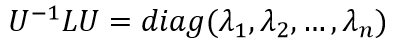
where λ ‘s are the corresponding eigenvalue of the eigenvectors. Let’s assume v is one of the columns of U which means it is one of the eigenvectors of L. Than it is not difficult to show the below equation in case of the unweighted graph[3].
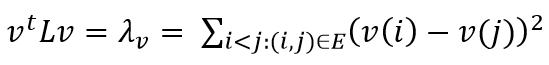
In the case of the weighted graph, the formula becomes as follows[5].
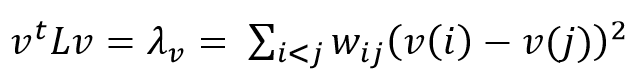
That equation is the most important point of Graph Embedding. Hence that formula tells us; if we assign the values of the eigenvector, whose eigenvalue is minimum, to the nodes as a value then the connected nodes value become as much as similar to each other. That is because of the left side of the formula which represents the square error of the connected node’s value (In case of the weighted graph the weights become weights of the square error). But if we assign the same value to every node, then the error becomes absolutely zero which we can obtain the trivial solution which is not our main target. Hence that formula tells us the error is also equal to the concerned eigenvalue, which means all eigenvalues must be positive and the one who is zero gives us a trivial solution where its eigenvector all consist of the same values. Hands-on again, Let’s calculate eigenvalues and eigenvectors of given Laplacian matrix and plot first three(smallest eigenvalues) eigenvectors.
% calculate basis
[u v]=eig(L);figure;
subplot(1,3,1);plot(u(:,1));ylim([-0.15 0.15]);xlim([1 101]); title(['1st eigenvector, value=' num2str(v(1,1))]);subplot(1,3,2);plot(u(:,2));ylim([-0.15 0.15]);xlim([1 101]); title(['2nd eigenvector, value=' num2str(v(2,2))]);subplot(1,3,3);plot(u(:,3));ylim([-0.15 0.15]);xlim([1 101]); title(['3th eigenvector, value=' num2str(v(3,3))]);
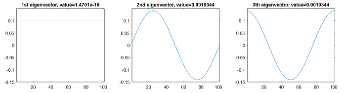
As you can see the eigenvector whose eigenvalue is zero gives a trivial solution as all nodes have the same value where the reason is obvious. But an interesting point is the eigenvector whose value is not zero but again as minimum as possible. For instance, as you can see 2nd and 3rd eigenvector’s values which change slightly from one node to its precedent node. Since we connected the first node to the last, also the last value and the first value of that eigenvector are just slightly different from each other which makes the square error minimum. The error values of 2nd and 3rd eigenvector (eigenvalues) are also the same for our case which is 0.001934.
This fact is the main logic behind the embedding the graph, which means map the node of the graph in some lower dimensional space such as 2D. So if we want to put those nodes into some location in 2D space, we should assign the minimum non-zero eigenvalue’s eigenvector for the 1st axis, the second minimum non-zero eigenvalues' eigenvector for the 2nd axis. The question is; what if we assign the maximum valued eigenvectors as locations of the nodes?
Here is the code for assigning the mentioned values to the coordinate of nodes and visualize it. Note we used GSPBox [4] to illustrate the graph and we just represent 21 nodes graph in order to avoid the complexity of figure.
%% show graph and signal
run ../gspbox/gsp_start
coor=u(:,2:3);
G=gsp_graph(W,coor);
figure;gsp_plot_graph(G)coor=u(:,end-1:end);
G=gsp_graph(W,coor);
figure;gsp_plot_graph(G)
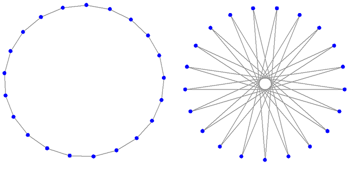
The embedding of the given time series graph using the first two non-zero valued eigenvectors amazingly makes sense. Putting all nodes around the circle nearby near is the best solution for the graph where the nodes just connected with its precedent and ancient nodes. As you guess using two eigenvectors whose eigenvalues are maximum is not good at all, vice versa it is the worst embedding. Again the nodes are located around the circle but connected nodes are as much as far away from another node. Now let’s have a look at all eigenvectors and their measured frequency for the same graph but n=101.

Fourier Transform versus Eigenvector Transform
Thanks to the Discrete Fourier Transform (DFT), we can rewrite any signal (1d,2d or nd having some special shape or just a noise does not matter) with the weighted sum of basis sinus signals (0Hz, 1Hz, 2Hz,….n/2Hz of sinusoidal signals for 1d case). The weight of each basis signal is a complex number where the magnitude of that weight shows the contribution of the basis signal, but the angle of that weight shows the phase of the basis signal. For the case of n=101 nodes time series signal, DTF result consists of 51 complex numbers (0hz to 50hz) the first coefficient represents the contribution of 0Hz sinus signal, but the last coefficient represents 50Hz sinus signal.
Interestingly, in Fig4, we can see that first eigenvector is just a line and its frequency is just 0. Second and third eigenvector are just 1 Hz sinusoidal signal but has 90-degree phase differ. Forth and fifth eigenvectors are 2Hz sinusoidal but have again 90-degree phase differ. And last two eigenvectors are 50Hz sinusoidal signal again 90-degree phase differ. So this fact encourages us to write the signal on the graph as the weighted sum of those bases (eigenvectors). But the coefficients must be a real number instead of complex in classical Fourier transform. Because we cannot guaranty that basis are perfectly sinus signal and we cannot shift them on the time domain in order to create phase difference. So instead of using 51 different sinus signal and change its phase if it is necessary to obtain the given input signal, we can use one 0Hz signal plus pair of signal and its already shifted by 90-degree form for i=1 to 50 (which makes 1+50x2=101 number of basis signal) to rewrite the given input signal. This process can be called Eigenvector Transform. In our case where the graph is a time series, we can know each eigenvector’s frequency. But in general case, we cannot know which frequency can be carried by each eigenvector. Even an eigenvector might carry a mixture of signals, we just know that these signals are an orthogonal basis and even so we can use that basis to rewrite our given input signal by the following equation where s is given signal and f is frequency profile. The second part refers to spatial to frequency transform, but the first part refers to the frequency to spatial transform.

In classical Fourier transform, we can represent the result by the magnitude of the basis versus the frequency of the basis and we called it frequency profile of the signal. But in general the graph signal case (not specifically our example for time series graph) we can just be sure that eigenvalues all positive and starts 0 and it monotonically increases. The minimum eigenvalue shows the minimum variation (sum of square differences of connected nodes value) of the value of connected nodes, maximum eigenvalue shows the maximum variation of the value of connected nodes, like how the first component of classical Fourier transform shows minimum frequency basis (just zero frequency stable straight line signal, the bias of the signal), the last component shows the magnitude of maximum frequency basis (the most variating signal which has as much as possible up and down)
So the best way to show the frequency profile for graph signal is using that extracted coefficient versus eigenvalue. Here is generated random signal s, it’s frequency profile (DFT results) and graph frequency profile.
% create arbitrary signal
s=randn(size(W,1),1);% calcualte graph frequency profile
f=u'*s;% calculate classical frequency profile
cf=abs(fft(s));
cf=cf(1:51);figure;subplot(1,2,1);plot(v,f,'r*-');
xlabel('eigenvalues');ylabel('coefficient');
title('Graph Frequency profile');subplot(1,2,2);plot(0:50,cf,'b*-');
xlabel('Frequencies');ylabel('magnitude');
title('Frequency profile');
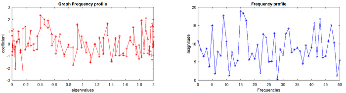
In classical frequency profile, there are 51 magnitude values (always positive since it is the absolute value of the complex number) where refers 0Hz to 50Hz for n=101 sampling point signal, but also that numbers have angle values as well which we did not plot it on the figure. But Graph Frequency profile consists of 101 real number and some might be negative. Because they are just a coefficient of the corresponding eigenvectors (Note negative coefficient means making the eigenvector signal up-down, which is equivalent of 180-degree phase differences).
Filtering on Frequency Domain
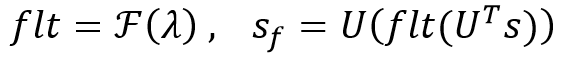
Classical frequency profile and graph frequency profile does not similar to each other. But we do not expect to get the same profile, hence orthogonal basis is different. But in our special time series graph case, we theoretically know that 1st eigenvectors frequency is 0Hz, 2nd and 3rd is 1Hz, 4th and 5th is 2Hz, and 100th and 101th is 50Hz. So if we create a frequency domain filter for classical signal, we can rewrite that filter coefficient for graph frequency profile and create our flt variable easily. Suppose somehow we write the graph filter flt by the function of eigenvalues, then filtered signal sf can be calculated by the following equation.
Here is the code of filtering the same random signal by classical frequency filter and graph frequency filtering where we use exp(-|f|/10) low pass filter.
% create filter for classical signal processing
fs=fftshift(fft(s));
f=linspace(-(n-1)/2,(n-1)/2,n)';
flt = exp(-abs(f)*0.1);% apply that filter on to time series signal
ot=ifft(ifftshift(flt.*fs));% create the same filter for graph signal processing
flt=[1:(n-1)/2]';
flt=[flt flt]';
flt=[0; flt(:)];
flt = exp(-abs(flt)*0.1);% apply that signal on to graph signal
sf=u*(flt.*(u'*s));% show results
figure;hold on;plot(s,'k--');plot(ot,'b-','linewidth',2);
xlim([1 n]);plot(sf,'r-','linewidth',1);
xlabel('node order or time');plot(ot-sf,'g-');
legend({'original signal','graph filtering','time series filtering','differences'});
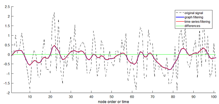
As a result, as long as we rewrite the filter for graph signals, we take the same results as you can see in the above figure. Actually, we do not need to find the same effect of the classic filter for graph signal in the application. I just did it to show the equivalent of both filtering techniques as a validation step. Normally we can create our own filters according to the eigenvalues. In the beginning, we told that even this signal is ordinary time series, we pretend it as comes from the graph. So here is the input and the filtered signal on the graph.
Graph Signal Filtering for 2D Euclidian Domain
So far, we have shown and validated the Graph signal filtering for 1D time series. Now we repeat the procedure for 2D euclidian signals such an image. Here is W matrix definition of the image whose size is 21x21.
n=21;
W=zeros(n*n,n*n);
for i=1:n
  for j=1:n
    p=sub2ind([n n],i,j);
    try
      p1=sub2ind([n n],i+1,j);
      W(p,p1)=1;
      W(p1,p)=1;
    catch
    end
    try
      p2=sub2ind([n n],i-1,j);
      W(p,p2)=1;
      W(p2,p)=1;
    catch
    end
    try
      p3=sub2ind([n n],i,j+1);
      W(p,p3)=1;
      W(p3,p)=1;
    catch
    end
    try
      p4=sub2ind([n n],i,j-1);
      W(p,p4)=1;
      W(p4,p)=1;
    catch
    end
  end
end
% connect left column to right column top rows to bottom row
for i=1:n
  p1=sub2ind([n n],1,i);
  p2=sub2ind([n n],n,i);
  W(p1,p2)=1;
  W(p2,p1)=1;
  p1=sub2ind([n n],i,1);
  p2=sub2ind([n n],i,n);
  W(p1,p2)=1;
  W(p2,p1)=1;
end
With the same procedure, we can calculate the Laplacian matrix, its eigenvalue, and eigenvectors.
% calculate Laplacian Matrix
d = sum(W,2);
L = diag(d)-W;% calculate basis
[u v]=eig(L);
% make eignevalue as vector
v=diag(v);
Here are all 21x21=441 eigenvectors and their dominant x and y-direction frequencies at the below figure.
As you can see again the first eigenvector is just plain image whose 2 direction frequency is just 0, then coming eigenvectors frequencies start to increase for both directions, till the last eigenvector has 10Hz for x-direction and 10Hz for the y-direction frequency which is the maximum frequency that 21x21 sampled 2D signal can carry. Again we created a random image and applied a certain low-pass filter on that image both two way and reported the results. Here is the code.
% generate random iamge
s=randn(n,n);% calculate centered frequcy of given image
F=fftshift(fft2(s));
[U V]=meshgrid(-fix(size(F,2)/2):fix(size(F,2)/2),-fix(size(F,1)/2):fix(size(F,1)/2));
UV=sqrt(U.^2+V.^2);
flt=exp(-1*UV);% filter image in frequency domain
FD=F.*flt;% transform the filtered image in to spatial domain
ot=ifft2(ifftshift(FD));% create similar filter for graph filterin
fltg=zeros(n*n,1);
for i=1:n*n
  i1=GG(i,2);
  j1=GG(i,3);
  fltg(i,1)=flt((n+1)/2+j1,(n+1)/2+i1);
end % apply filter on graph signal
sf=u*(fltg.*(u'*s(:)));% report results
figure;subplot(2,2,1);imagesc(s);axis image;title('Input image');subplot(2,2,2);imagesc(ot,[-0.05 0.2]);axis image;title('Classic Filtering Result');subplot(2,2,3);imagesc(reshape(sf,[n n ]),[-0.05 0.2]);axis image;title('Graph Signal Filtering Result');subplot(2,2,4);imagesc(reshape(sf,[n n ])-ot);axis image;title('Differences');
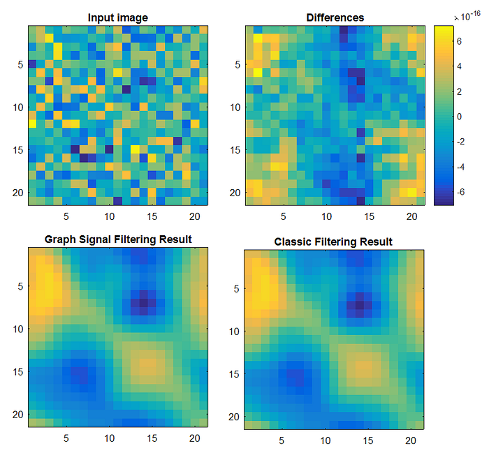
Again the results are similar. But we do not need to find the equivalent filter of both cases. We just need to define our filter as a function of eigenvalues.
Interesting things for a graph representation of 2D euclidian domain signal is the graph embedding. If in our W matrix definition, we get connected the leftmost column pixels to the rightmost column but cut the connection of the most up line pixels to the most bottom-line pixel. Here is the result of graph embedding and the filtered signal on it.
Graph Signal Filtering for Non-Euclidian Domain
Now time to make something valuable. We have a connected, undirected any graph where it has 100 nodes and node’s predefined locations. The graph is a weighted graph so W matrix consists of 0 or positive real numbers. Here is loading predefined graph and eigenvector calculations.
clear all% load predefined W matrix for 100 nodes
load mydata% calculate Laplacian Matrix
d = sum(W,2);
L = diag(d)-W;% find eigenvector and eigenvalues of Laplacian
[u v]=eig(L);% make eignevalue as vector
v=diag(v);% get maximum eigenvalue
lmax=max(v);
Now we need to define a filter. Let's do it again low pass filter by the following equation.
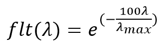
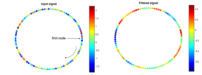
This definition is definitely low pass filter. Since if the lower λ values the function’s output become high. (for 0 input it gives 1 output) but for higher λ values the output becomes low. So that function passes low frequency but suppresses high frequency. We want to apply that filter where the signal on the graph is all zero but just 1st node signal is 1. Here is the code for signal definition, filter definition, applying it on to the Graph signal and visualization of the results.
% create signal where first node is 1 rest of them 0
s=zeros(size(W,1),1);
s(1)=1;% define filter
flt =exp(-100*v/lmax);% apply that filter on to graph signal
sf=u*(flt.*(u'*s));% visualize input and result
G=gsp_graph(W,coord);
figure;gsp_plot_signal(G,s);title('Input signal');
figure;gsp_plot_signal(G,sf);title('Filtered signal');
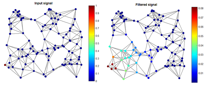
The result seems extremely logical. Hence just the one node has high value but the rest of them is zero, we expected from low-pass filter to spread that value around and make the signal blur. The result is exactly what we expected.
Graph Embedding According to Node Distance
Another interesting feature of the Laplacian Matrix and its Eigenvectors is weighted Graph embedding as long as connected node distances are known, but there is no location information. In this case, we can use again minimum non-zero eigenvalues' eigenvectors to estimate the positions of the nodes by the minimum square error solution. To demonstrate that feature first nodes over the circle created but the distance of the consecutive nodes is random. After we set the connected nodes weight as w(i,j)=w(j,i)=1/d(i,j) . Here are the codes.
% create time series grid as graph
n=101;
W=zeros(n,n);
ang=linspace(0,2*pi,10*n);
p=randperm(length(ang));
p=sort(p(1:n));p=[p p(1)];
for i=1:n+1
  loc(i,:)=[cos(ang(p(i))) sin(ang(p(i)))];
endfor i=1:n-1
  d=norm(loc(i,:)-loc(i+1,:));
  W(i,i+1)=(1/d);
  W(i+1,i)=(1/d);
endd=norm(loc(1,:)-loc(n,:));
W(1,n)=(1/d);
W(n,1)=(1/d);
W=W/max(W(:));
Then again Laplacian and eigenvector calculations.
% calculate Laplacian Matrix
d = sum(W,2);
L = diag(d)-W;% calculate basis
[u v]=eig(L);
v=diag(v);
Signal creating and reporting code.
% create arbitrary signal
s=1:n;
% show graph and signal
G=gsp_graph(W,loc(1:end-1,:));
figure;gsp_plot_signal(G,s)
title('original coordinates ');G=gsp_graph(W,u(:,2:3));
figure;gsp_plot_signal(G,s)
title('esimated coordinates');du=diff(u(:,2:3));
dt=diff(loc(1:end-1,:));
figure;plot(diag(du*du'),diag(dt*dt'),'r.')
xlabel('estimated ');ylabel('actual ');
title('consecutive node distance');
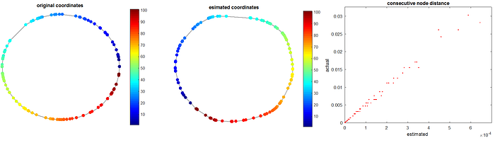
The result is not perfect but pretty good. Also, actual consecutive node distance and estimated node distances are almost linear. This result encourages us to use a weighted graph representation for euclidian signal where the sampling rate is variable.
What is Next?
So far the mechanism of graph signal processing is mostly figured out. That is the logic behind the Spectral Graph Neural Network which is one of the graph CNN methods. This method basically applies the filters on frequency domain instead of classical CNN usage as a spatial domain filter. The next step must be figuring out spatial filtering on graph signals.
Note
This research was funded by LITIS Lab at University of Rouen-Normandy. It is part of AGAC Project (Projet Régional RIN Recherche sur l’analyse de graphes et ses applications à la chemoinformatique).
You can find the demo code on my GitHub profile.
References
[1] Grassi, Francesco, et al. “A time-vertex signal processing framework.” arXiv preprint arXiv:1705.02307 (2017).
[2] Marsden, Anne. “Eigenvalues of the Laplacian and Their Relationship to the Connectedness of a Graph.” University of Chicago, REU (2013).
[3] Roughgarden, Tim, and Gregory Valiant. “CS168: The Modern Algorithmic Toolbox Lectures# 11 and# 12: Spectral Graph Theory.” (2016).
[4] Perraudin, Nathanaël, et al. “GSPBOX: A toolbox for signal processing on graphs.” arXiv preprint arXiv:1408.5781 (2014).
[5] Poignard, Camille, Tiago Pereira, and Jan Philipp Pade. “Spectra of Laplacian matrices of weighted graphs: structural genericity properties.” SIAM Journal on Applied Mathematics78.1 (2018): 372–394.